NetProVis

Telecom networks are moving from dedicated hardware boxes to cloud-native network functions (CNFs): firewalls, gateways, load balancers and DNS servers running as containers on Kubernetes. That brings elasticity, but only if the autoscaling is tuned well. Set the threshold too low and you pay for idle replicas. Set it too high and traffic spikes hit before new pods are ready.

Kubernetes’ Horizontal Pod Autoscaler (HPA) scales on a fixed utilisation target, say 70% CPU, chosen by a human once and rarely revisited. NetProVis asks: what if the target itself adapted, based on a forecast of where the workload is heading?

What it does

NetProVis is a full-stack web application for Google Kubernetes Engine (GKE):

• Sign in with Google (OAuth 2.0), then pick a GCP project and cluster.
• Deploy CNFs in one click from Helm charts: Kong gateway, Airlock firewall, NGINX load balancer, Falco IDS, OpenVPN, CoreDNS, RabbitMQ and Prometheus monitoring. Each has its own CPU and memory requests and limits.
• Monitor cluster CPU, memory and per-node network ingress and egress in real time.
• Turn on adaptive HPA per workload, for CPU, memory or both.
• Review history and reports. Every threshold change is logged and charted against actual usage, and can be exported as a PDF report.

The adaptive autoscaling loop

1. Cloud MonitoringLast 80 min of request utilisation, 1-min means
2. Forecast serviceLSTM on Cloud Functions
3. ThresholdNew target utilisation %
4. Kubernetes APICreate or update autoscaling/v2 HPA

When a user enables adaptive HPA on a workload, the FastAPI backend schedules a job for it with APScheduler. The job runs once immediately, then every minute:

@app.post("/activate_hpa")
async def activate_hpa(p: Pod):
    pod = json.loads(p.selected_pod)
    job_ids = [f"adaptive_hpa_job_for_{pod['metadata']['name']}_{res}"
               for res in (['cpu', 'memory'] if p.resource_type == 'all' else [p.resource_type])]

    for job_id in job_ids:
        resource = job_id.split('_')[-1]
        if not scheduler.get_job(job_id):
            scheduler.add_job(adaptive_hpa, 'interval', minutes=1,
                              args=[pod, resource, project, cluster], id=job_id)
            await adaptive_hpa(pod, resource, project, cluster)

Each run pulls the workload’s recent request utilisation from Google Cloud Monitoring as one-minute means over the last 80 minutes. It sends that series to a forecasting model deployed as a Cloud Function, which returns the utilisation target to use next:

async def adaptive_hpa(pod, resource_type, pod_project, pod_cluster):
    resource_request_utilization = await get_resource_request_utilization(
        project_id, cluster_name, cluster_zone, pod, resource_type)
    threshold_value = await fetch_forecast_threshold(resource_request_utilization)

    res = await create_hpa(cluster_endpoint, "cnf-namespace", pod_name,
                           pod.get('kind', ''), threshold_value, resource_type)

    # Keep a rolling history (max 100 points) for the threshold charts
    past_thresholds.setdefault(pod_name, {}).setdefault(resource_type, {}) \
        .setdefault("thresholdValues", []).append({get_current_date(): threshold_value})

The new target is written straight to the cluster through the Kubernetes REST API as an autoscaling/v2 HPA. The first run creates it; on a 409 Conflict the existing HPA is updated instead. CPU and memory metrics are merged into the same HPA, so enabling one never overwrites the other:

def generate_payload(pod_name, pod_type, threshold_value, resource_type, existing_hpa_metrics):
    payload = copy.deepcopy(HPA_TEMPLATE)
    payload['metadata']['name'] = f"adaptive-hpa-for-{pod_name}"
    payload['spec']['scaleTargetRef'].update({'kind': pod_type, 'name': pod_name})

    # Update the existing metric's target, or append a new one
    existing = any(m['type'] == 'Resource' and m['resource']['name'] == resource_type
                   for m in existing_hpa_metrics)
    if existing:
        for m in existing_hpa_metrics:
            if m['type'] == 'Resource' and m['resource']['name'] == resource_type:
                m['resource']['target']['averageUtilization'] = int(threshold_value)
    else:
        existing_hpa_metrics.append({
            "type": "Resource",
            "resource": {
                "name": resource_type,
                "target": {"type": "Utilization", "averageUtilization": int(threshold_value)},
            },
        })

    payload['spec']['metrics'] = existing_hpa_metrics
    return payload

If anything in the loop fails, the job unschedules itself and logs the reason to the task feed. A broken forecast should never leave a workload with a half-applied scaling policy. On shutdown, the backend deletes every HPA it created, so the cluster returns to its original state.

Forecasting load with an LSTM

The forecast service is where the ML happens. It is a TensorFlow/Keras model served as an HTTP Cloud Function (forecast_http): the backend posts a utilisation series as JSON and gets back a threshold.

I chose a Long Short-Term Memory (LSTM) network because resource usage is a time series, and what happens next depends on what happened over the last hour, not just the last minute. A plain RNN loses that context quickly. An LSTM’s input, forget and output gates let it keep longer-range patterns, such as a load that has been climbing steadily, while ignoring one-off noise.

The forecasting pipeline works in these steps:

1. Prepare. Clean the timestamped utilisation metrics and fill in missing values.
2. Scale. Normalise values to the 0–1 range with MinMaxScaler, which LSTMs train on much more reliably than raw percentages.
3. Window. Slice the series into supervised pairs. Each input is N_LOOKBACK = 84 past one-minute points, and each target is the next N_FORECAST = 24 points.
4. Train. Fit a model of LSTM and Dense layers in Keras, tuning the LSTM units, activations and optimiser. EarlyStopping stops training when validation loss stops improving, and ModelCheckpoint keeps the best weights, so the model doesn’t overfit.
5. Forecast. Feed the most recent 84-point window into the model to predict the next 24 minutes.
6. Invert. Transform the forecast back from the 0–1 scale to utilisation percentages.
7. Evaluate. Measure accuracy with mean absolute percentage error (MAPE).

So each call turns 84 minutes of history into a 24-minute look ahead. That lead time is the point: the threshold can move before the load arrives, rather than after the HPA has already fallen behind.

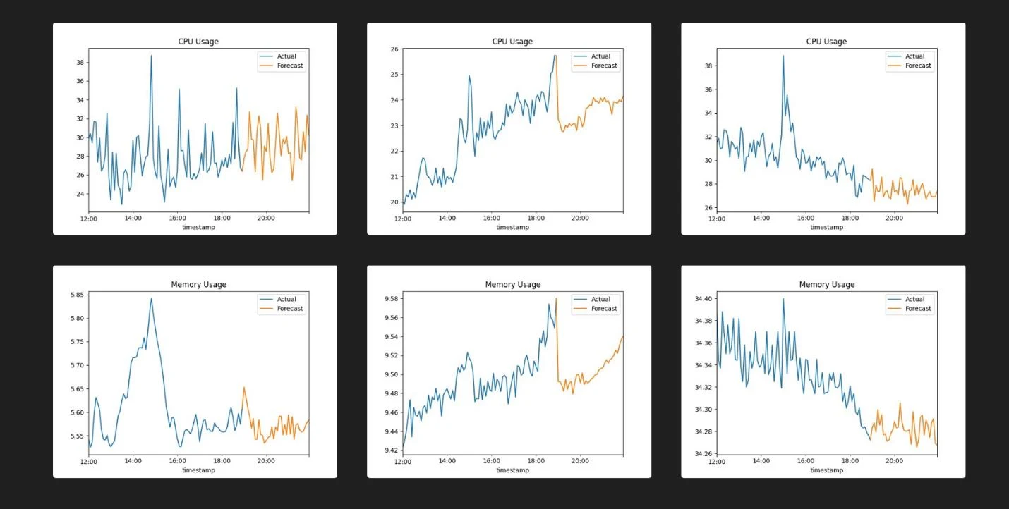
The forecasts track the overall direction of each series well, including a steady CPU climb and a gradual decline, but they are smoother than reality. Sudden spikes, like the memory jump in the first memory chart, are mostly not predicted. For autoscaling that is a reasonable trade: the HPA should follow sustained changes in load, not chase every blip.

From forecast to threshold

A forecast is not yet a scaling policy. A small decision algorithm, calculate_threshold, turns the 24 forecast points into a single HPA target:

1. Weight by recency. Weights decrease linearly across the forecast, so the next few minutes count more than the end of the 24-minute horizon, where the forecast is least certain.
2. Summarise. Compute the weighted mean and the weighted standard deviation of the forecast. The standard deviation captures how volatile the coming load looks.
3. Combine. The threshold is (mean + std) × 1.5. The multiplier is a tunable sensitivity knob.
4. Clamp. Keep the result between 30% and 85%. Below 30%, the HPA would scale on almost any activity. Above 85%, new pods would arrive too late for a spike.

Splitting the work like this kept each part simple to reason about. The LSTM only predicts usage, and the policy lives in a few lines of arithmetic that can be tuned without retraining anything.

Testing the forecast service

I tested the service with generated JSON datasets that mimic patterns seen in a live cluster: steady, high, low, oscillating and erratic loads. Then I compared the threshold it chose against each load.

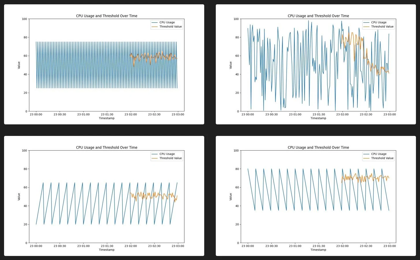
Across the patterns, the threshold stayed much steadier than the load. On regular oscillations it settled near the middle of the range instead of following every peak. On erratic load it moved in broad steps. This is the behaviour you want from an autoscaler: responsive to real shifts in demand, but not so twitchy that it thrashes pods up and down. It lagged slightly behind very sharp drops, which errs on the side of keeping capacity a little longer.

I also load-tested real CNFs on GKE with Apache JMeter and BusyBox, with adaptive HPA turned on.

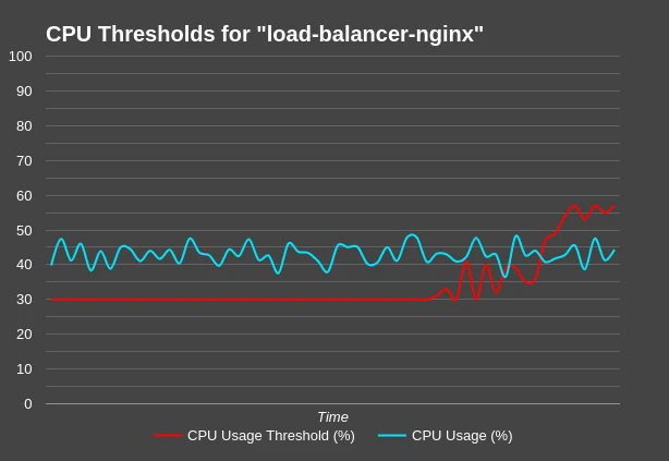
On the NGINX load balancer, CPU usage hovered between 40% and 50%. The threshold started at the 30% floor, which would have kept extra replicas running, and climbed to 55–60% as the forecasts came in. The load balancer stayed responsive throughout, with fewer replicas than the static low target would have used.

Deploying network functions

CNFs are deployed with Helm. The backend maps each function to a public chart, applies the user’s resource requests and limits, and replaces any existing release of the same name:

helm_install_cmd = [
    "helm", "install", cnf_name, chart_name, "--set",
    f"resources.limits.cpu={params['cpuLimit']},resources.limits.memory={params['memoryLimit']},"
    f"resources.requests.cpu={params['cpuRequested']},resources.requests.memory={params['memoryRequested']}",
    "--namespace", "cnf-namespace",
]

Because every CNF lands in a dedicated cnf-namespace, the dashboard detects them automatically by namespace. No manual registration is needed.

The dashboard

The React front-end (Google Charts) shows cluster-wide CPU and memory, per-node network traffic, running workloads and a live task feed. Its most useful view for evaluation is Threshold Stats, which plots the HPA target the model chose against the workload’s actual usage over time. That makes it easy to see whether the autoscaler is leading the load or lagging behind it.

Results

Compared with a static HPA target, the forecast-driven thresholds reduced resource cost by 5–10% on fluctuating workloads.

Adaptive HPA is not free, though. A fixed target is predictable and easy to reason about, which suits steady workloads. The adaptive one depends on a model’s view of the future, so it is less transparent, and it can still miss sudden spikes that the LSTM smooths over. The next steps I identified were feeding the model network-level signals such as latency and packet loss, and improving the model and decision algorithm so they react better to abrupt changes.

What I took away

This project sat at the intersection of ML and infrastructure, and the hard parts were mostly on the infrastructure side: authenticating against GKE and Cloud Monitoring, querying time-series data correctly, and making a control loop that can fail safely. The lesson was that a prediction is only useful if the system acting on it is robust. Idempotent updates, cleanup on failure and a visible history of every decision mattered as much as the model.